 |
| Web-Schrödinger
3.3 |
(C)2007-2021 G. I.
Márk, Ph. Lambin, L. P. Biró, EK MFA Budapest,Hungary --
Uni Namur, Belgium
www.nanotechnology.hu |
|
|
|
Subscribe to
the mailing list to receive E-mail news about Web-Schrödinger (new
versions. etc)
Watch introductory
videos
from the Web-Schrödinger YT channel.
Introduction
Web-Schrödinger is a program for the interactive solution of
the stationary (time independent) and time dependent two dimensional
(2D) Schrödinger
equation. The program itself runs on our server and can be used
through the Internet with a simple Web browser (Internet Explorer,
Mozilla, Opera, Chrome was tested). Nothing is installed on the user's
computer. The user can load, run, and modify ready-made example files,
or prepare her/his own configuration(s), which can be saved on her/his
own computer for later use.
See
[1]
for a detailed description of the program.
Theoretical background
Time dependent Schrödinger equation
The time evolution of the quantum mechanical wave function ψ(r;t)
is governed by the time dependent Schrödinger equation:
where r = (x,y) is the
position coordinate, t is the time and H
= K + V is the Hamilton
operator, K is the operator of the kinetic
energy, and V = V(x,y) is the
operator of the potential energy.
When the potential function V(x,y) and the initial wave
function ψ(x,y,t0) = ψ0(x,y) is known,
the time dependent Schrödinger equation determines the wave
function ψ(x,y,t) for any time value. We can calculate all
observables from the wave function, for example the rho(x,y,t)
probability density and the j(x,y,t) probability
current density.
Stationary Schrödinger equation
rho(x,y,t) gives the probability of finding the quantum
mechanical particle around the point (x,y)
at time t. We call those ψ(x,y,t)=ψ(x,y)
states, where ψ(x,y) is independent of time, stationary
states. The stationary (time independent) states are given by the
stationary Schrödinger equation:
Hψ(r) = Eψ(r)
where E is the energy of the state.
User
Guide
All functions of the program are available through a menu system.
Upon starting the program a default configuration is loaded, the user
can immediatelly run this through the Calculation
menu, or load
another configuration with the Load
Example, or Load menu
points. All
parameters can be modified in the Edit
menu and the current setup can
be saved anytime with the help of the Save
function.
Menu system
Files
Load Example
We have prepared several characteristic examples, illustrating the
most important phenomena of quantum mechanics, including the spreading
of the wave packet, tunneling, bound states, etc. The current list of
the examples is given in Appendix A. The example library is
continuously expanding, see Appendix A for
the up to date status. After loading an example setup the user can
study and modify the parameters through the Edit menu or go straight to Calculation to calculate the time
development and/or the stationary states.
Load
This function makes it possible to load the user's own configuration
files, from her/his own computer. Such parameter files can be created
either by saving a (possibly modified) example configuration (or the
default configuration) or writing a configuration file from the scratch
with a text editor or any other program.
Save
The current state of the parameters can be saved anytime to the
user's own computer.
Edit
Mesh
The wave function and the potential is represented on a 2D mesh.
Here you can specify the number of mesh points (Nx , Ny)
in the x and y direction and the size of the
calculation region in Angström (sx, sy).
For
typical
applications
the
Δx = sx/Nx, Δy
= sy/Ny values should be between 0.1 - 1
Å. The origin of the coordinate system is in the middle of the
calculation region.
The numerical algorith uses a periodic boundary condition, i.e. what
goes out of the calculation region at the right side, comes in at the
left side. It is like if the whole plane were "tiled" with the
calculation region. As a consequence when the wave packet approaches
the boundary of the calculation box, it "meets" its copy at the
neighboring box and this causes unphysical interference effects to
appear in the probability density. The parameters of the calculation
(spatial- and temporal mesh, potential, and initial state) should be
carefully chosen to avoid this effect.
V0 gives the default value of the potential in
eV (Electronvolt).
Note: due to the difference of the algorithms used for the solution
of the time dependent and stationary Schrödinger equations,
generally a finer mesh is necessary for the time dependent calculation.
E.g. a Nx=256 is typical
value for the time dependent, and Nx=64
for
the
stationary
calculation
Potential
The potential V(x,y) can be interactively assembled from
objects of several types: circle, rectangle, and plane.
Any
number
of
these
objects
can
be
given.
For
each
object
the
user
can
specify
its
geometrical parameters and its potential value. For pixels
where several objects overlap, the object given most recently
determines the pixel potential value. The program shows the potential
function generated from the current set of objects as a grayscale
image.
- The potential for the circle is defined by:
V(r) = V0 + V1 r + V2 r2
- The potential for the plane is defined by:
V(d) = V0 + V1 d + V2 d2,
where d is the (perpendicular) distance from the boundary line
- The potential for the rectangle is defined by:
V(x,y) =
V0 +
Vx x + Vy y +
Vxx x2 + Vyy y2 +
Vxy x y ,
where x and y are the (perpendicular)
distances from the x and y sides of the rectangle
Initial state
Here the user can specify the initial wave function ψ0(x,y),
which
is
the
input
of
the
time
dependent
calculation
(it
is not used at
the stationary calculation).
Its
general
form
is
a so called truncated plane wave [8] wave packet, i.e. a Gaussian
wave packet convolved with a 2D square window function. The program
displays the chosen initial state together with the potential function,
as a composite color image. In order to ensure that the wave packet has
its ideal form (minimal size and flat envelope) when it hits the
potential, a time retardation procedure is included into the initial
state preparation. The user can specify the retardation time by giving
the the bx, by distance
values, which mean that after proceeding such distances in x,
and y the wave packet should have its "ideal" form.
ax, ay give the spatial
width of the wave packet. The initial state should be specified such a
way, that its overlap with the potential objects is negligible.
Detectors
The user can place horizontal or vertical line segments (detectors)
into the calculation window. The program calculates the probability
current I(t) passing through
each line segment during the time evolution of the wave packet and also
its time integral T for the
whole calculation time. T is
called transmission, because it gives the probability that the quantum
particle crosses the given line segment (detector).
Calculation parameters
Here we can specify the parameters of the time dependent and the
stationary
calculation.
Parameters used for the time
evolution calculation: The number of time points is Nt
and Δt
gives calculation time step. Δt has to be given in atomic
time units, 1 au time = 0.0242 fs (femtosecond).
The numerical algorithm imposes a condition on the maximal Δt
value that can be used: Δt < 4/π (Δx)2 / D,
where
D is the number of dimensions, D=2 in 2D.
(This formula is valid in atomic units, i.e. one has to insert Δx
in Bohr, 1 Bohr = 0.529 Å. For the default Δx =
0.3
Å, Δt = 0.2 au is suitable and this is the
default time step.)
It is not necessary, however, to display the results in such a fine
time scale. Therefore the user can input the "display timestep", i.e.
the number of calculation time steps, when the wave function is
displayed.
Parameters used for the stationary
calculation: Nstat
gives the number of states calculated.
Calculation
Time development
When the user hits the "RUN" button, the time development
calculation starts on the server. The progress of the calculation is
shown by small thumbnail images. For typical parameters the time
development calculation takes 1-2 minutes. (If there are more
concurrent jobs on the server – either from this user or from others –
the calculation may be somewhat slower. The program writes out the
number of concurrent jobs – if there is any – after hitting the "RUN"
button.)
Eigenstates
When the user hits the "RUN" button, the calculation of the stationary
states starts on the server. It takes several second, or minutes,
depending on the mesh size, and the number of orbitals requested. (If
there are more
concurrent jobs on the server – either from this user or from others –
the calculation may be somewhat slower. The program writes out the
number of concurrent jobs – if there is any – after hitting the "RUN"
button.) When the calculation is completed, the program displays the
energies and the wave functions of the stationary states.
Results
After the time development calculation is completed on the server,
the time development of the probability density is displayed in
composite color images. The program first calculates the global maximum
of the probability and normalizes each frame using this value. A
nonlinear color scale (γ=2.5) is used in order to facilitate
presentation.
If the user placed detectors into the calculation window before the
start of the calculation, the program also displays the I(t) probability current functions
and T transmission values for
each of the detectors.
Appendix A:
Examples
The examples are diveded into two groups: examples for time development
calculation and examples for stationary states calculation. Nothing
prevents to perform both a time evolution and a stationary states
calculation for the same example, but those examples listed under "time
development" demonstrate interesting cases of time development, those
listed under "stationary states" demonstrate interesting cases of
eiegenstates. For some cases, however, e.g. for a potential box, both
the time evolution and the stationary states gives instructive results.
The examples were carefully designed to prevent the effect of the
periodic boundary condition. For the time evolution examples, this was
accomplished by halting the time development calculation before the
wave packet reaches the edge of the calculation box. For the stationary
states calculation, we applied a potential wall at the edges in each
examples.
Examples for time development calculation
band_1D_allowed
A wave packet is approaching a periodic potential with energy in the
allowed band. The wave packet is passing through the potential.
band_1D_forbidden
A wave packet is approaching a periodic potential with energy in the
forbidden band. The wave packet is reflected from the potential.
Christmas
Wave packet scattering on a potential forming a Christmas tree
gravity
Quantum analogue of a projectile motion.
Wave packet scattering on a linearly increasing potential.
The "Results" menu shows the transferred probabilities and probability densities
crossing the detectors shown by the red line segments.
hardcore
Scattering of a wave packet on a circular hardcore potential. Note the
circular component of the final state.
quantum_revival
Demonstration of the "quantum revival" phenomenon.
stm_on_nanotube
Simulation of Scanning Tunneling Microscope imaging of a carbon
nanotube. See [4]
for details..
tunneling_oblique
Tunneling of a wave packet through a potential wall of V>E. The WP
is hitting the wall at 75o angle.
tunneling_perpendicular
Tunneling of a wave packet through a potential wall of V>E. The WP
is hitting the wall az 90o angle.
two_balls
Two colliding billiard balls on a 1D track, shown in 2D configuration space. For more explanation, see
this video.
Comparison of an experiment, a classial mechanics- and quantum mechanics simulation of two colliding billiard balls on a one-dimensional track. Introduction of the concept of configuration space. Comparison of two-particle states for interacting- and non-interacting particles. Two-particle states for interacting particles show Wigner-crystal-like behavior.
two_pendulums
Two coupled pendulums, shown in 2D configuration space.
Examples for stationary states calculation
box
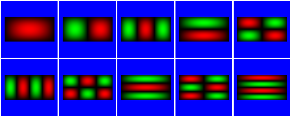
Eigenstates of a rectangular potential box.
circle
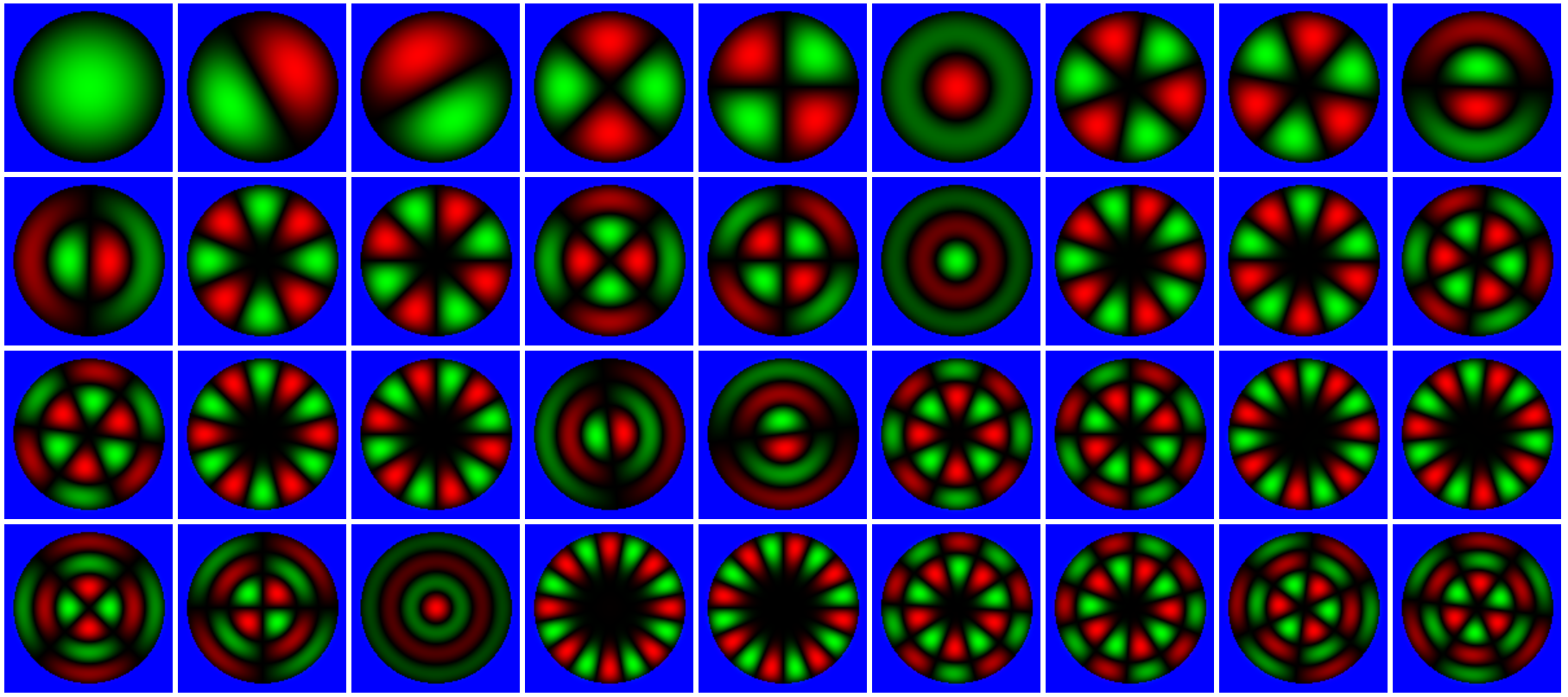
Eigenstates of a circular potential box.
harmosc_2d
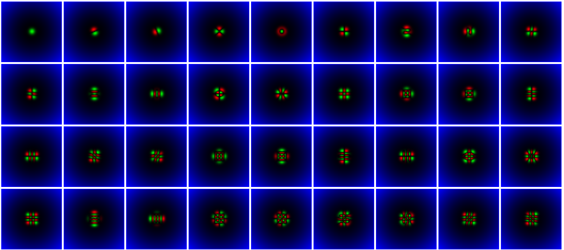
Eigenstates of a two-dimensional radial quadratic potential.
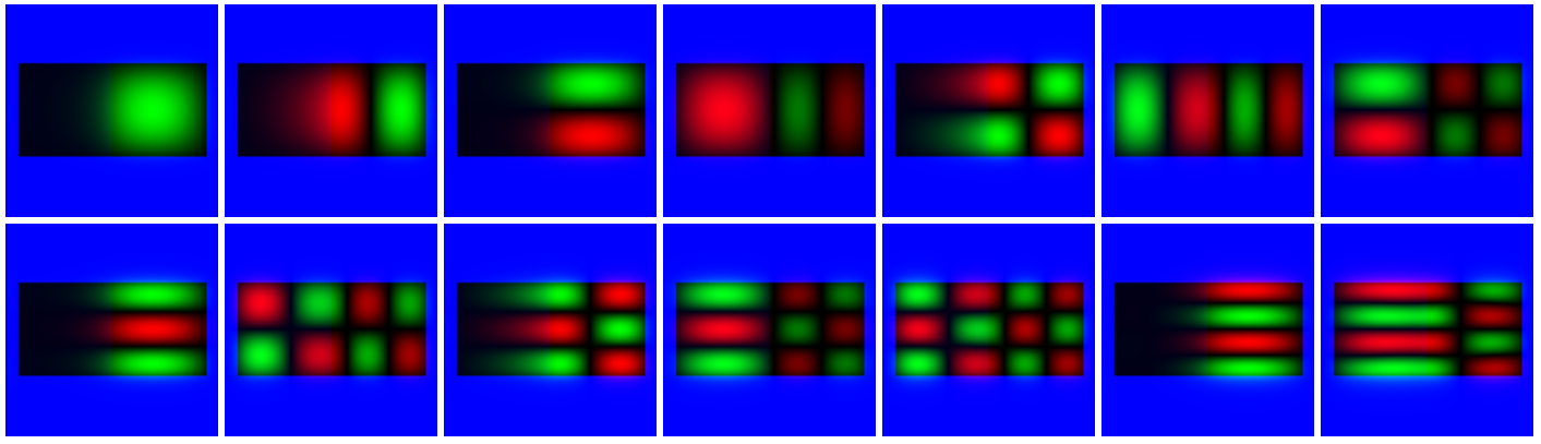
molecule
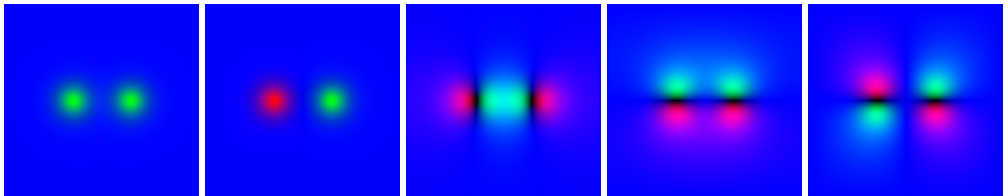
Eigenstates of a simple model for a diatomic molecule.
Note the two lowest orbitals are "s" like orbitals, similar to the atomic orbitals,
the third orbital is a "sigma" orbital, and the fourth and fifth orbitals are
"pi" orbitals.
step
This includes a potential step inside a potential box: the left half of
the potential has a slightly higher potential value than the righ half.
Example
file contest
Develop your own example files demonstrating interesting quantum
phenomena! You can send the SAVE-d files to mark@mfa.kfki.hu . Best
example files will be included into the Web-Schrödinger "Examples"
directory. Please attach also a brief description of the example!
Mailing list
We have a mailing list for announcing new features and examples.
The mailing list is hosted by Google Groups.
-
If you want to subsribe using a GMail address, then simply
click here.
-
If you want to join the mailing list using a non-GMail address, then
send an E-mail to
web-schroedinger+subscribe@googlegroups.com
from the address that you want to be subscribed.
You will receive an email asking you to click to confirm.
Do not do that, as then you'll find the subscribing email address
changed to that of your Google account.
Instead, reply to the confirmation email.
It doesn't matter whether your reply has any content.
Then you should receive a further email, to your chosen address, saying that you are subscribed.
At this point you probably can't change any options, etc., via the web interface.
You can unsubscribe using the same procedure with
web-schroedinger+unsubscribe@googlegroups.com .
References
-
Márk, Géza, I.:
Web-Schrödinger: Program for the interactive solution of the time dependent and stationary two dimensional (2D) Schrödinger equation;
arXiv:2004.10046 [physics.ed-ph] (2020)
https://arxiv.org/abs/2004.10046
- Schrödinger equation; (in several
languages)
http://en.wikipedia.org/wiki/Schroedinger_equation
- Time development of quantum mechanical systems; (1995-)
(English and Hungarian)
http://www.kfki.hu/~mark/physedu/schrodinger/index.html
-
Márk,
Géza, I.; Biró, László, P.; Gyulai,
József: Simulation of STM images of 3D surfaces and
comparison with experimental data: carbon nanotubes;
Phys. Rev. B 58, 12645(1998).
http://www.nanotechnology.hu/reprint/prb_58_12645.pdf
-
Márk, Géza, I.; Biró, László,
P.; Gyulai, József; Thiry, Paul, A.; Lucas, Amand, A.; Lambin,
Philippe: Simulation of scanning tunneling spectroscopy of
supported carbon nanotubes;
Phys. Rev. B 62, 2797(2000).
http://www.nanotechnology.hu/reprint/prb_62_2797.pdf
- Lambin, Philippe; Márk, Géza, I.; Meunier, Vincent;
Biró, László, P.: Computation of STM images
of carbon nanotubes;
Int. J. Qunatum.. Chem. 95,
495(2003).
http://www.nanotechnology.hu/reprint/IntJQuantChem_95_493_STMSimul.pdf
- Márk, Géza, I.; Biró, László,
P.; Lambin, Philippe: Calculation of axial charge spreading in
carbon nanotubes and
nanotube Y-junctions during STM measurement;
Phys. Rev. B 70,
115423-1(2004).
http://www.nanotechnology.hu/reprint/prb_70_115423_3d.pdf
- Géza I. Márk PhD
Thesis, FUNDP Namur, 2006.
http://www.mfa.kfki.hu/~mark/phd/index.html
- Márk, Géza, I.; Vancsó, Péter; Hwang,
Chanyong; Lambin, Philippe; Biró, László, P.:
Anisotropic dynamics of charge
carriers in graphene;
Phys. Rev. B 85,
125443-1(2012).
http://www.nanotechnology.hu/reprint/prb_85_125443_graphene_anisotropy_2012.pdf
- Vancsó, Péter; Márk, Géza,
István; Hwang, Chanyong; Lambin, Philippe; Biró,
László, P.:
Time and energy dependent
dynamics of the STM tip – graphene system;
European Journal of Physics B 85,
142-1(2012)
http://www.nanotechnology.hu/reprint/epjb_85_142_graphene_jellium_2012.pdf
- Márk, Géza, I.; Vancsó, Péter;
Lambin, Philippe; Hwang, Chanyong; Biró, László,
P.:
Forming electronic waveguides
from graphene grain boundaries;
Journal of Nanophotonics 6,
061719-1(2012)
http://www.nanotechnology.hu/reprint/jnanophot_6_061718_waveguide2012.pdf
- S. Janecek, E.
Krotscheck: A fast and simple
program for solving local Schrödinger equations in two and three
dimensions;
Comput. Phys. Comm. 178 (11) (2008) 835–842.
http://www.sciencedirect.com/science/article/pii/S0010465508000453
- S.A. Chin, S. Janecek, and E. Krotscheck: An arbitrary order diffusion algorithm for
solving Schrödinger equations;
Computer Physics Communications 180 (2009) 1700–1708.
http://www.sciencedirect.com/science/article/pii/S0010465509001131
Last updated: February 4, 2021 by Géza I. Márk ,
mark@mfa.kfki.hu
This page was accessed  times since Feb 8, 2013.